When we have a transformation from one state \(x_t\) to another \(x_{t+1}\): \[ x_{t+1} = U x_t \] where \(U\) is a unitary matrix. In the case of 3 qubits, \(U\) is \([8, 8]\). \[ U = \begin{bmatrix} a_{00} & a_{01} & a_{02} & a_{03} & a_{04} & a_{05} & a_{06} & a_{07} \\ a_{10} & a_{11} & a_{12} & a_{13} & a_{14} & a_{15} & a_{16} & a_{17} \\ a_{20} & a_{21} & a_{22} & a_{23} & a_{24} & a_{25} & a_{26} & a_{27} \\ a_{30} & a_{31} & a_{32} & a_{33} & a_{34} & a_{35} & a_{36} & a_{37} \\ a_{40} & a_{41} & a_{42} & a_{43} & a_{44} & a_{45} & a_{46} & a_{47} \\ a_{50} & a_{51} & a_{52} & a_{53} & a_{54} & a_{55} & a_{56} & a_{57} \\ a_{60} & a_{61} & a_{62} & a_{63} & a_{64} & a_{65} & a_{66} & a_{67} \\ a_{70} & a_{71} & a_{72} & a_{73} & a_{74} & a_{75} & a_{76} & a_{77} \\ \end{bmatrix} \]
Quantum Interference
When we talk about quantum interference in quantum computing, what are we talking about?
My idea originates from the Double Slit Experiment. In the experiment, there are two slits. In my view, there’s one
“qubit” in the experiment. A photon can go through either one of the slits or both of them in superposition. Two base
states
|1> and |0> interfere with each other due to the phase difference that is caused by the difference of traversed
distances.

Figure 1: Double Slit Experiment
Figure from Wikipedia.
If we have 3 qubits in our quantum computer, we have 8 base states, then we have 8 conceptual slits in our experiment.
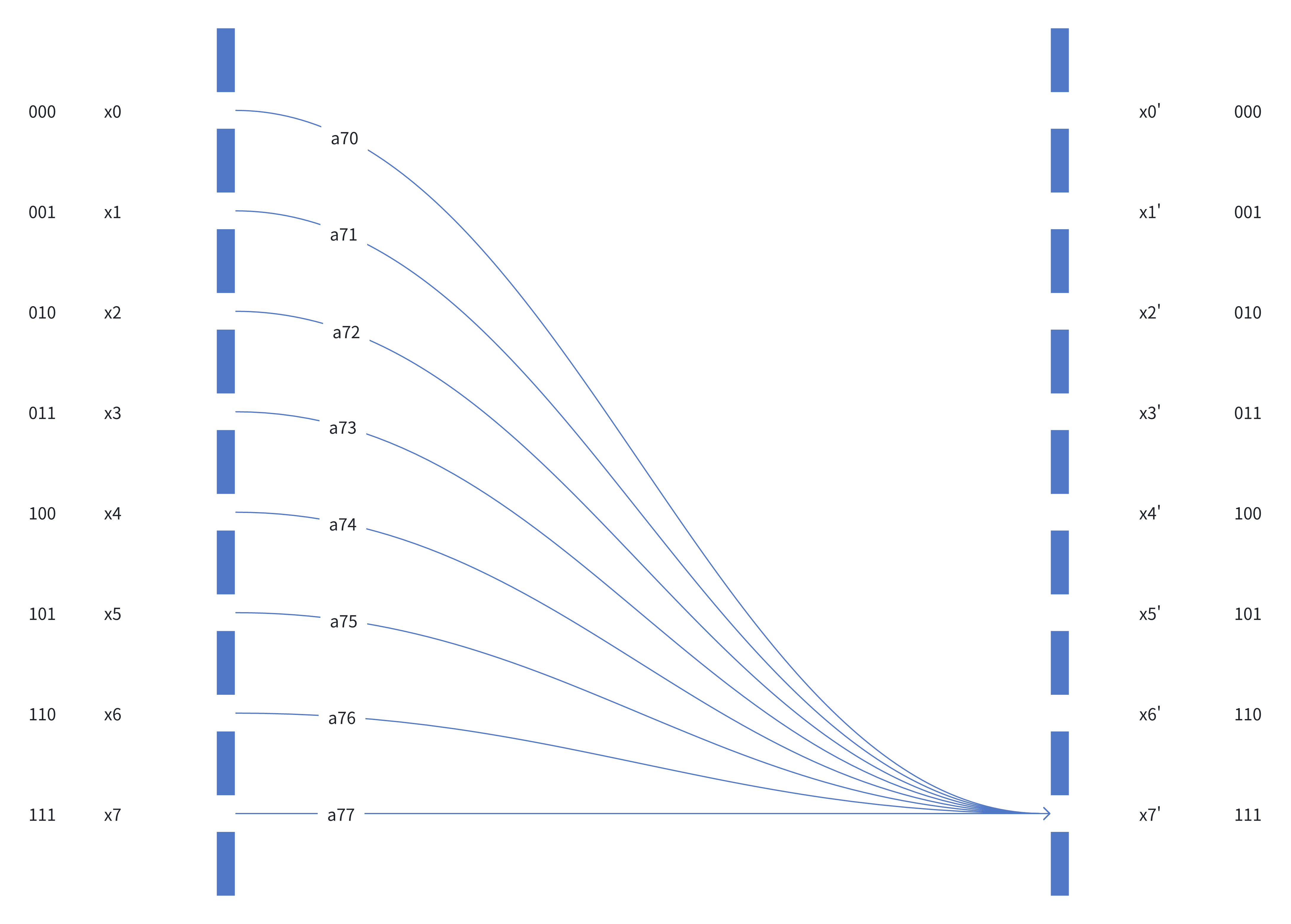
Figure 2
Conceptually, there are 8 start states and 8 end states.
The end states are discrete rather than in a continuum in the Double Slit Experiment.
For the 7th entry of \(x_{t+1}\), denoted as \(x_7'\), its value is \[ x_7' = \sum_{i=0}^7 a_{7i} x_i \]
Equation 1, in which \(a_{7i}\) is the entry (7, i) of \(U\) and \(x_i\) is the i-th entry of \(x_t\).
Phase and Amplitude in a Physical Sense
From Euler’s Formula: \[ e^{i\theta} = cos\theta + sin\theta i \] any complex number \(y\) can be represented as \[ y = Ae^{i\theta} = a + bi \\ A = \sqrt{a^2+b^2} \\ a,b,\theta \in \mathbb{R} \] where \(A\) is the amplitude of \(y\).
So, for \(y_1, y_2 \in \mathbb{C}\) \[ y_1\cdot y_2 = A_1 A_2\ e^{(\theta_1 + \theta_2) i} \] where \(\theta_1 + \theta_2\) is the change in phase, \(A_1 A_2\) in amplitude.
So, in the Equation 1, \(a_{7i} x_i\) describes how each of the base states changes in terms of phase and amplitude, with respect to \(x_7'\), as demonstrated by each curved line in the figure.
Take \(a_{70}x_{0}\) as an example, in physical sense, it means how the amplitude and phase will change when the base
state |000> “traverses” through the “environment” and reaches the base state |111>. The “environment” is defined
by \(U\).
Interference with a Vector Interpretation
A complex number is a vector in the complex plane. With this interpretation, multiplication of two complex numbers is the actions of stretching (i.e., amplitude change) and rotation (i.e., phase change).
So, each term in the Equation 1, \(a_{7i} x_i\) , is stretching and rotating \(x_i\) by \(a_{7i}\), yielding a new vector.
Let’s denote \(a_{7i} x_i\) as \(v_i\). \[ x_7' = \sum_{i=0}^7 a_{7i} * x_i = \sum_{i=0}^7 v_i \]
Graphically we have

To measure the contribution of each \(v_i\) to \(x_7'\), we can do projection like done by real-valued vector product.
Suppose: \[ x_7' = (a, b) \\ v_7 = (k, j) \] the contribution of \(v_7\) is \[ c_7 = \frac{ak + bj}{\sqrt{a^2 + b^2}} \] The illustration is shown below:

In this case, \(c_7\) is a negative number, meaning the base state |111> at \(t\), after traversing through the
“environment” defined by \(U\), negatively impacts the probability / amplitude of base state |111> at \(t+1\).
Visualization
With this contribution measure, we can define a function to calculate all the contributions likewise, giving a contribution matrix \(C\).
\[ C = f(U, x_i) \]
\[ C = \begin{bmatrix} c_{00} & c_{01} & c_{02} & c_{03} & c_{04} & c_{05} & c_{06} & c_{07} \\ c_{10} & c_{11} & c_{12} & c_{13} & c_{14} & c_{15} & c_{16} & c_{17} \\ c_{20} & c_{21} & c_{22} & c_{23} & c_{24} & c_{25} & c_{26} & c_{27} \\ c_{30} & c_{31} & c_{32} & c_{33} & c_{34} & c_{35} & c_{36} & c_{37} \\ c_{40} & c_{41} & c_{42} & c_{43} & c_{44} & c_{45} & c_{46} & c_{47} \\ c_{50} & c_{51} & c_{52} & c_{53} & c_{54} & c_{55} & c_{56} & c_{57} \\ c_{60} & c_{61} & c_{62} & c_{63} & c_{64} & c_{65} & c_{66} & c_{67} \\ c_{70} & c_{71} & c_{72} & c_{73} & c_{74} & c_{75} & c_{76} & c_{77} \\ \end{bmatrix} \]
\[ x_j' = \sum_{k} i_{jk} * x_k = \sum_{k} v_{jk} = m + ni \\ v_{jk} = a + bi \\ c_{jk} = \frac{am + nb}{\sqrt{m^2 + n^2}} \]
This matrix can be visualized like confusion matrices.
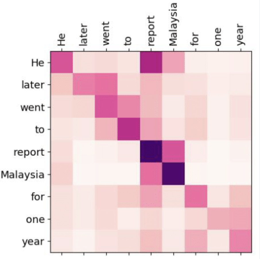
Figure 3: An example of confusion matrices in the context of NLP
Such visualization can be applied similarly to \(C\), where the color scheme illustrates the sign and magnitude of contribution of each entry.
For a base state to stand out, the corresponding row of \(C\) should be almost of the same color (contributions); if the corresponding row of \(C\) is full of different colors, the contributions to a base state cancel out.
Figure 2 can also be enhanced if the color of a line indicates contribution.
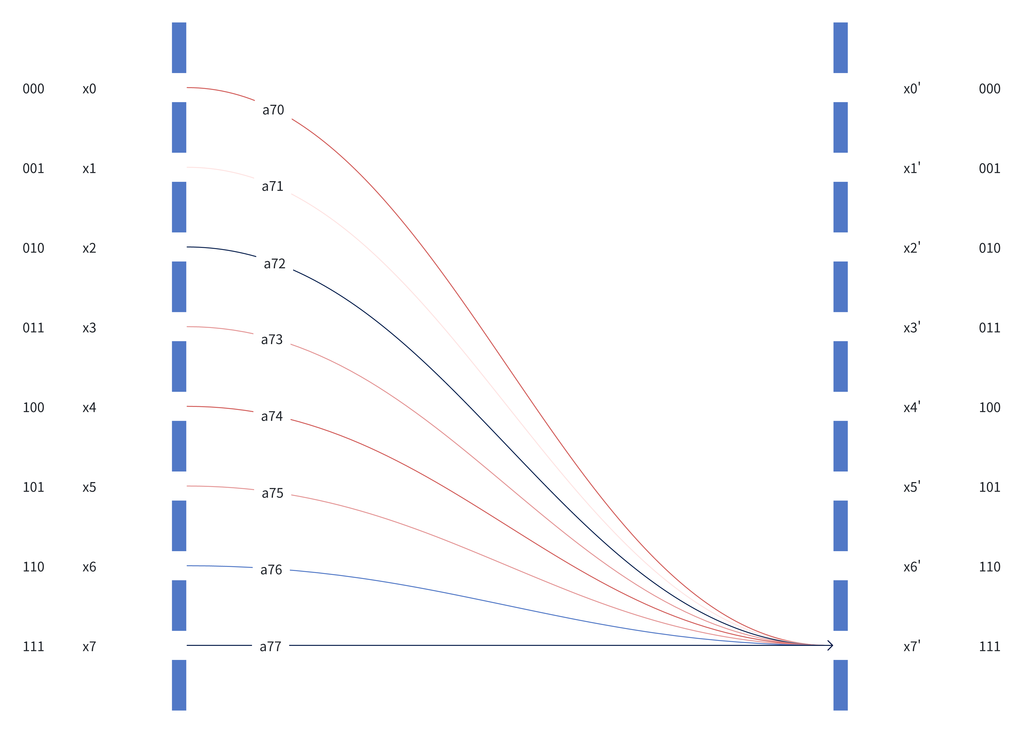
Figure 4: Figure 2 enhanced with a color scheme
Red: Positive Contribution
Blue: Negative Contribution
Scalability
Such visualization of \(C\) can be easily scaled to 10-qubit systems, in which \(C\) is a 1024x1024 matrix that can be displayed on a modern monitor.
We can group base states by grouping qubits and summing their respective contributions. For example, we can group qubits as qubytes, then the visualization scale is reduced by 256 times. This is equivalent to binary subdividing \(C\) into submatrices and then summing up their entries.
For example, if we group the last \(k=2\) of 3 qubits, the expanded view of \(C\) is like below:
\[ C = \begin{bmatrix} \begin{bmatrix} c_{00} & c_{01} & c_{02} & c_{03} \\ c_{10} & c_{11} & c_{12} & c_{13} \\ c_{20} & c_{21} & c_{22} & c_{23} \\ c_{30} & c_{31} & c_{32} & c_{33} \\ \end{bmatrix} & \begin{bmatrix} c_{04} & c_{05} & c_{06} & c_{07} \\ c_{14} & c_{15} & c_{16} & c_{17} \\ c_{24} & c_{25} & c_{26} & c_{27} \\ c_{34} & c_{35} & c_{36} & c_{37} \\ \end{bmatrix} \\ \begin{bmatrix} c_{40} & c_{41} & c_{42} & c_{43} \\ c_{50} & c_{51} & c_{52} & c_{53} \\ c_{60} & c_{61} & c_{62} & c_{63} \\ c_{70} & c_{71} & c_{72} & c_{73} \\ \end{bmatrix} & \begin{bmatrix} c_{44} & c_{45} & c_{46} & c_{47} \\ c_{54} & c_{55} & c_{56} & c_{57} \\ c_{64} & c_{65} & c_{66} & c_{67} \\ c_{74} & c_{75} & c_{76} & c_{77} \\ \end{bmatrix} \end{bmatrix} \]
The compressed view of \(C\) has only 4 entries, so the compress ratio is 16 (\(=2^k\times 2^k\)) times (from 64 to 4).
Such visualization can scale to (10+8) qubit systems by grouping by qubytes. With hierarchical grouping, the visualization can also scale beyond (10+8) qubit systems.